Searching With QWAK

Here, we will go over the searching algorithm using QWAK for several different structures.

Complete Graph

Single Element

To use QWAK for searching, we need to define a graph for the search space, and the targets are marked elements, specified as a list of weighted node indices. For a complete graph, the optimal transition rate is \(\gamma = \frac{1}{n}\), resulting in a search time of \(\mathcal{O}(\sqrt{N})\), comparable to Grover’s algorithm.

n = 200
t = (np.pi/2) * np.sqrt(n)
gamma = 1/n
init = list(range(0,n))
graph = nx.complete_graph(n)
qw = QWAK(graph, gamma=gamma, markedElements=[(n//2, -1)],
          laplacian=False)
qw.runWalk(t, initStateList=init)

Firstly, we initialize QWAK with the desired simulation parameters, so that we can calculate the search problem via the runWalk method. Because we created the object with a list of marked elements, the Hamiltonian of the method will be described as:

\[H^\prime = -\gamma A - \sum_{x \in M} \ket{x}\bra{x}\]

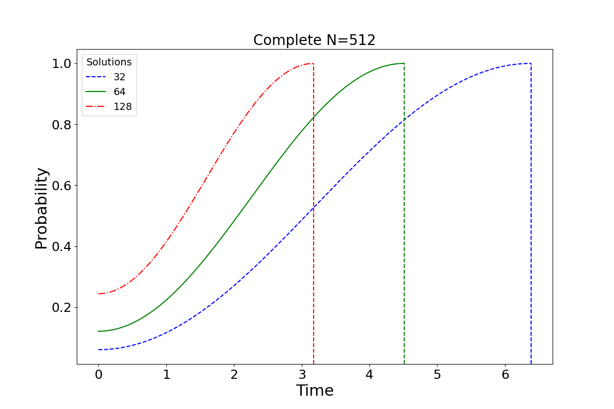
The optimal time for the search problem also depends on the number of solutions, and the previous figure presents the evolution of the sum probability of all the marked elements. The utility functions needed to plot this figure are available in the package.

Multiple Elements

markedElements = [(n//2,-1),(n//2+1,-1)]
t = (np.pi/2) * np.sqrt(n/len(markedElements))

To search for multiple elements, we simply extend the markedElements list and fine-tune the optimal evolution time. The aforementioned figure demonstrates that as the number of marked elements increases, the time required to reach maximum probability decreases. Specifically, when we mark \(\frac{1}{4}\) of the total elements, the walk evolves optimally in time \(\pi\). This scenario is analogous to the single-shot Grover algorithm, where the highest probability for finding the solution is achieved in just one step.

Hypercube

The \(n\)-dimensional hypercube is a graph of \(N=2^n\) vertices, where two vertices will be connected if one differs only in a single bit from the other.

The evolution of the search problem over this structure presents a sharp transition at a critical value of \(\gamma\), given by

(1)\[\gamma_{\text{opt}} = \frac{1}{2^n} \sum_{r=1}^n \binom{n}{r} \frac{1}{r} = \frac{2}{n} + O\left(n^{-2}\right)\]

Here, we attempt to showcase that the maximum probability of the solution is indeed sensitive to the transition rate. For this purpose, we create a QWAK object for each value of \(\gamma\), and then we evolve the walk in a time interval with the runMultipleWalks function.

n = 9
gamma = gamma_hypercube(n)
graph = nx.hypercube_graph(n)

N = 2**n
t = (np.pi/2) * np.sqrt(N)
mElem = [(N//2, -1)]
initSL = list(range(0,N))
probDistMat = []

for gamma in gammaList:
    qw = QWAK(graph=graph, gamma=gamma,
              initStateList=initSL, markedElements=mElem)
    qw.runMultipleWalks(timeList=tList)
    probDistMat.append(qw.getProbDistList())

The probability distribution matrix is composed of lists of ProbabilityDistribution objects, for each value of \(\gamma\). We now generate a plot to visualize the search process and the effect of different values of \(\gamma\) on the probability of finding the marked element. The plot is shown in the following figure, obtained with auxiliary functions available in the notebook.

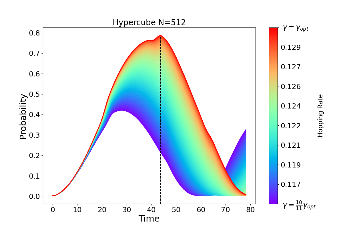
We can see from the plot that despite having a very narrow range of transition rate values, \(\gamma_{\text{opt}}\) does indeed reach maximum probability within time that scales with \(\mathcal{O}\sqrt{N}\).

Erdős-Rényi model

As a final example, we will examine the search problem on a more general collection of random graphs. In the Erdős-Rényi (ER) model, a graph is constructed by starting with a fixed number of nodes and then connecting each pair of nodes with a fixed probability \(p\). As a consequence, the model produces graphs with varying degrees of connectivity and randomness, depending on the chosen value of \(p\).

However, it has been shown that search by CTQW is optimal for almost all graphs, given the correct conditions. To explore the behavior of the search process in these structures, we will perform a series of simulations with varying parameters. First, we create a list of ER graphs with different connection probabilities.

N = 500
t = (np.pi/2) * np.sqrt(N)
samples = 200
pList = np.linspace(0.01, 0.5, samples)
graphList = [nx.erdos_renyi_graph(N, p) for p in pList]

Next, we initialize a QWAK object for each graph in the list and set a transition rate of \(\gamma = \frac{1}{N p}\). We will store the probability distributions in a matrix for further analysis.

initSL = list(range(0, N))
tList = np.linspace(0, 100, samples)
mElem = [(N//2, -1)]
probDistMat = []

for graph, pVal in zip(graphList, pList):
    gamma = 1/(N*pVal)
    qw = QWAK(graph=graph, gamma=gamma,
              initStateList=initSL, markedElements=mElem)
    qw.runMultipleWalks(timeList=tList)
    probDistMat.append(qw.getProbDistList())

Finally, we can visualize the results in the following figure by generating a heatmap plot, with the connection probabilities on the x-axis as a function of time in the y-axis. The color intensity represents the maximum probability of finding the marked element at each combination of parameters.

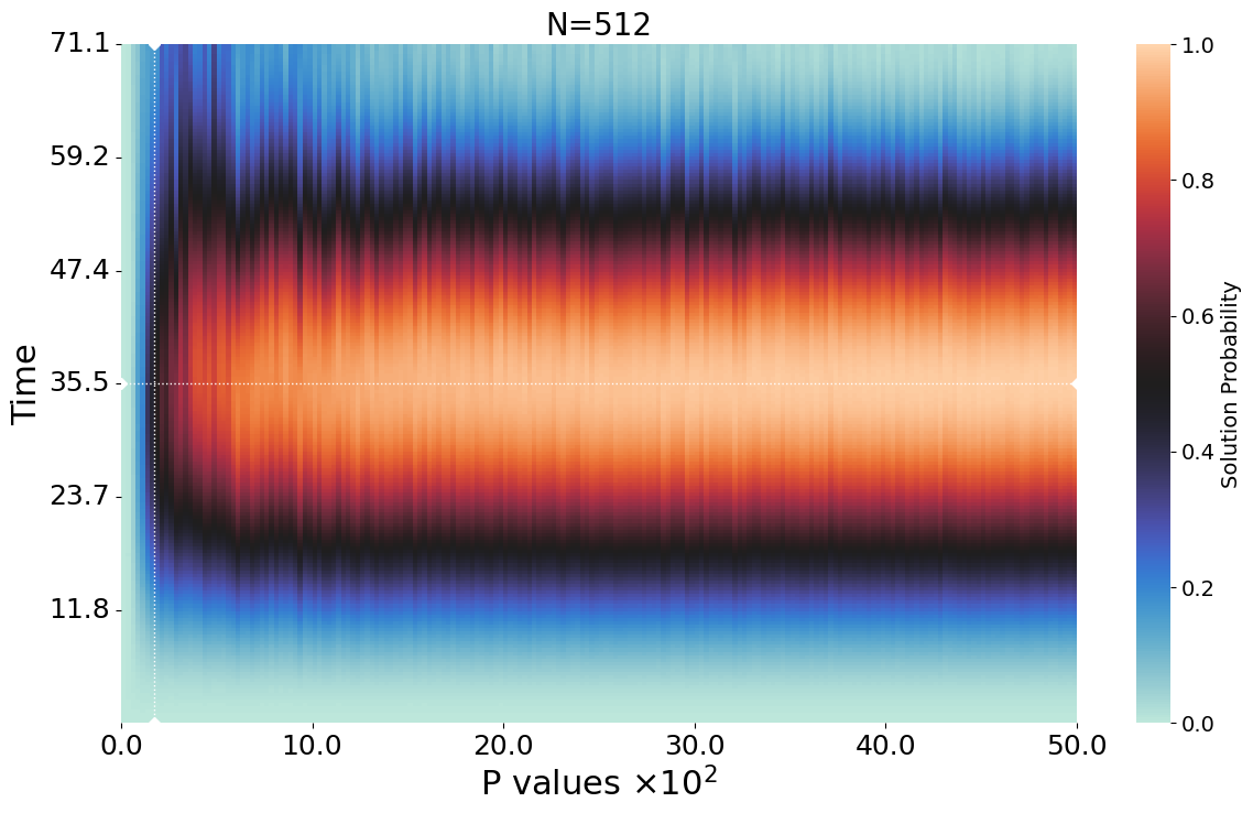
When the value of \(p\) in a graph exceeds the percolation threshold of \(p=\frac{\log{N}}{N}\), the graph is almost certainly connected. The figure highlights this threshold with a vertical line and shows that the search process achieves high solution probabilities above it, in time \(\mathcal{O}(\sqrt{N})\). For each value of \(p\), 40 different graphs were generated in order to calculate the average solution probability.