Directed Quantum Walk#
A directed graph \(G=(V,E)\) differs from its undirected counterpart by having ordered vertex pairs in \(E\). Early work established strong quadrangularity and graph reversibility as prerequisites for coined quantum walks (CQWs) on such graphs. Recent studies show performance gains in centrality ranking via CTQWs, with applications like PageRank. Other models, like staggered quantum walks, have also been defined in these structures.
Directed graphs exhibit distinct transport properties, requiring different methods to characterize state transfer. Additionally, these graphs can exhibit new phenomena, such as zero state transfer.
In the subsequent sections, we will demonstrate how to use QWAK for
simulating CTQWs on directed infinite lines and explore the enhanced
decay rate of the survival probability in more general
structures.
Dynamics#
To define a directed infinite line, as shown in the figure below, we use the Hamiltonian \(H\) given by equation
where \(L\) and \(R\) are the left and right borders of the line, respectively. We can obtain an infinite path graph by setting \(R\rightarrow\infty\) and \(L\rightarrow -\infty\).
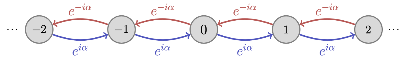
We implement the finite line using the path_graph function and add direction to it using
the getWeightedGraph function available in the notebook.
1n = 100
2alpha = np.pi/2
3weight = np.exp(1j*alpha)
4baseGraph = nx.path_graph(n, create_using=nx.DiGraph)
5graph = getWeightedGraph(baseGraph, weight)
Inspired by previous work, we choose a non-localized initial condition given by equation
which can be easily implemented in Python.
1k = 1
2theta = np.pi/4
3l = 0
4gamma = l * np.pi
5
6initCond = [(n//2-k, np.cos(theta)), (n//2+k, np.exp(1j*gamma)*np.sin(theta))]
After initializing the QWAK object, we
compute the walk using the runWalk method. To specify a
non-localized initial condition, we pass the customStateList parameter
to provide both the node and its corresponding amplitude.
1t = 35
2
3qw = QWAK(graph)
4qw.runWalk(time = t, customStateList = initCond)
5
6probVec = qw.getProbVec()
The probability distribution is obtained using the getProbVec method. To
study how the evolution of the probability distribution changes with different
graph weights, the following figure displays the CTQW
for multiple values of \(\alpha\).
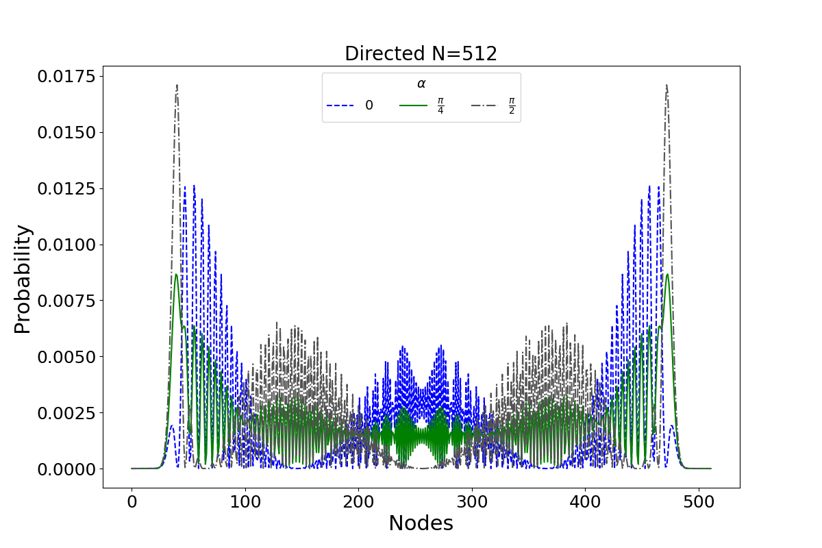
Indeed, the value of \(\alpha\) has a severe impact on the dynamics of the walk. In the case of an undirected graph (\(\alpha = 0\)), symmetry is expected around the center node; however, varying values of \(\alpha\) can alter the shape of the distribution, presenting a method of controlling how the walker propagates throughout the structure.
Survival Probability#
The survival probability of a quantum walk can be characterized as the mean probability of finding the walker in a certain location after some time \(t\). Considering the symmetric position range of \([k_0,k_1]\), this quantity will be
Here, we will use QWAK to run the walk for an interval using multiple
values of \(\alpha\). Classically, the survival probability decays at a rate
proportionate to \(t^{-\frac{1}{2}}\), while a quantum walk typically decays
quadratically faster at a rate of \(t^{-1}\). It is known, however, that certain
initial conditions can achieve enhanced decay rate, scaling with \(t^{-3}\).
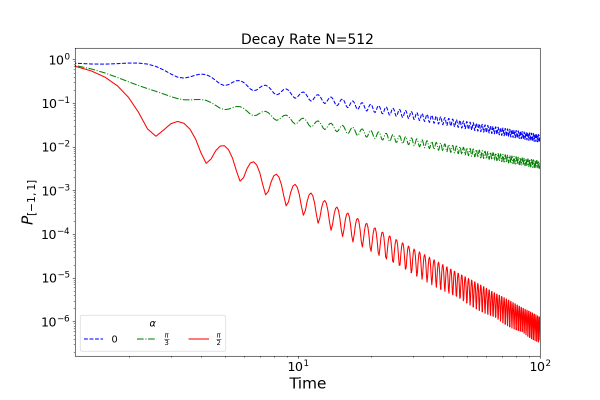
Using the previously defined directed graph and the chosen initial condition, we can analyze the impact of varying \(\alpha\) values on the decay rate of the survival probability:
 1timeList = np.linspace(0, 100, 500)
 2alphaList = [0, np.pi/3, np.pi/2]
 3decayRateMatrix = []
 4for alpha in alphaList:
 5    weight = np.exp(1j * alpha)
 6    graph = getWeightedGraph(baseGraph, weight)
 7    qw = QWAK(graph)
 8    qw.runMultipleWalks(timeList, customStateList=initCond)
 9    decayRateMatrix.append(
10                  qw.getSurvivalProbList(N//2 - k, N//2 + k))
11
12plt.loglog()
13for decayRate in decayRateMatrix:
14    plt.plot(survProbList)
15plt.show()
The code iterates through a list of \(\alpha\) values, generating a directed graph for each and computing the corresponding survival probabilities over time. These are stored in a decay rate matrix for log-log plotting, as shown in the previous figure.
Directional line graphs enable more effective control of interference effects in quantum walks. This allows for both normal and enhanced decay rates under broader initial conditions. The figure shows that an optimal \(\alpha\) value can be chosen to accelerate decay, irrespective of \(k\)’s parity.